Atmospheric Dispersion Characteristics of Radioactive Materials according to the Local Weather and Emission Conditions

1. Setting the local weather and emission conditions

In order to identify the most recurrent local weather conditions near the Kori Nuclear Power Plant (KNPP), a statistical method called cluster analysis was used based on the weather observation data collected within the surrounding areas of the KNPP. A representative date for modeling was selected based on the cluster analysis of the annual wind data of 2012 collected from 28 weather stations located within 60 km of the KNPP. The results of the cluster analysis showed that 4 clusters were statistically significant. For the cluster in which the most dates fell on, another cluster analysis was re-executed in order to subdivide it into 5 clusters. The 8 clusters that were finally categorized were labeled ME1, ME2, ME3, ME4_1, ME4_2, ME4_3, ME4_4, and ME4_5. While the ME1-3 clusters showed a consistent wind system under relatively strong synoptic weather conditions, the wind speed was weak for the ME4_1-5 clusters, where a time change in the local winds appeared. ME1 (representative date: December 8, 2012, cluster occurrence rate: 14.5%) was influenced by the winter monsoon of the Korean peninsula, so the daily mean temperature was 1.3°C lower with a high frequency of a strong northwesterly wind (3.2 m·s⁻¹ mean speed), and ME2 (March 12, 2012, 27.0%) had a high frequency of a north wind with a daily mean wind speed of 2.8 m·s⁻¹. For ME3 (June 25, 2012, 14.5%), there was precipitation before and after the representative date due to the influence of the rainy season, and a northeasterly wind was consistently observed. ME4_1 (May 18, 2012, 8.5%), ME4_2 (February 27, 2012, 9.8%), and ME4_3 (May 29, 2012, 7.7%) showed sunny days due to the influence of high atmospheric pressure in the Korean peninsula, and the daily mean wind speed was 2.4–2.8 m·s⁻¹, with directions of the main wind being south-southwest, north-northwest, and northeast-east, respectively. ME4_4 (May 8, 2012, 9.3%) and ME4_5 (September 5, 2012, 8.7%) were cloudy days or days with low precipitation due to low atmospheric pressure or because the Korean peninsula was located at the edge of high atmospheric pressure, and the daily mean wind speed was 2.7 m·s⁻¹ and 3.5 m·s⁻¹, respectively, with the direction of the main wind being south and west-southwest, respectively. Details of the cluster analysis and the weather conditions of the representative dates are presented in reference [4].

The emission conditions of radioactive materials were set after combining the emission rates and the total number of particles. The emission rate is defined by the amount of pollutants emitted from the source of pollution during a fixed period of time. A more objective time change of the ¹³⁷Cs emission rate was set using ¹³⁷Cs emission data for 24 hours based on 1) the emission rate [3] calculated from the Atmospheric Transport Model Evaluation Study for the Chernobyl nuclear accident (a case in which radioactive materials were almost consistently leaked every hour of every day after a hydrogen explosion) and 2) the emission rate [2, 8] calculated from observed data by Tokyo Electric Power Company (TEPCO) for the Fukushima nuclear disaster (a case in which a large amount of radioactive materials was leaked due to a hydrogen explosion following a radiation spill) (Figure 1). The total number of particles was composed so that a total of 1,000/10,000/100,000 imaginary particles would be emitted during the 24 hours after the start of the nuclear accident. A total of six types of emission conditions for radioactive materials were set by combining the two types of emission rates and the three types of particle numbers: EM1_1, EM1_2, EM1_3, EM2_1, EM2_2, and EM2_3. The emission rates and the number of particles per emission condition are presented in Table 1.

Fig. 1

Time variations of emission rate of ¹³⁷Cs from the Chernobyl nuclear accident case (blue dotted line) and the Fukushima nuclear accident case (red dotted line).

Table 1

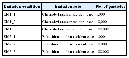
¹³⁷Cs Emission Rate and Number of Particles for Each Emission Condition

2. Forecast method for the dispersion of radioactive material outflow

Figure 2 is a summary of the forecast methods of radioactive material dispersion in this study. Based on HYSPLIT [9], a Langrangian particle diffusion model, the creation process of the main input data (topography, weather, and emission) was schematized. HYSPLIT calculates the transportation and dispersion process based on the Langrangian method [10] and can trace not only the concentration of the pollutant but also the normal direction and reverse direction trajectories of the pollutant. Compared to other atmospheric dispersion models, HYSPLIT has a smaller calculation volume and takes less time to calculate results. The modeling region of HYSPLIT was 100 km×100 km centering around the Kori Nuclear Power Plant and composed of 202×202 grids of 0.005m (approximately 500 m) horizontal resolution. The vertical grid was composed of 14 levels (0, 10, 20, 40, 80, 160, 300, 500, 1,500, 2,000, 3,000, 4,000, 5,000, 10,000 m from the ground surface). The modeling was carried out for 48 hours after a nuclear accident—which included representative dates per local weather condition—in order to analyze the atmospheric dispersion of radioactive materials.

Fig. 2

The flowchart for atmospheric dispersion prediction system of radioactive materials.

Conducting air dispersion modeling requires meteorological information (temperature, wind (components u and v), surface pressure, atmospheric boundary layer) on the modeling region during the modeling period. The numerical value per grid depending on the meterological factor is created through meteorological modeling. A meteorological model is used to forecast weather in regions where observation is not carried out or to forecast future weather. It is calculated through mathematical differentiation and appropriate physical approximation catered to the climate system based on basic laws of physics such as Newton’s law of motion. Various meterological models exist such as the Mesoscale Meteorological Model Version 5 (MM5), the Weather Research and Forecasting (WRF) model, and the Unified Model (UM). This study used the WRF (Ver. 3.5) model. The WRF model offers physical options that can implement numerical simulation of the latest technological advances and can be used for various purposes such as optimal simulation, parameterization, data assimilation, forecast research, combination between models, and real-time forecasting. The U.S. National Weather Service currently uses the WRF model, which is known to be highly efficient in mesoscale and regional weather simulation when compared to other meteorological models. The input data for initial/alert data of the WRF in this study used Final (FNL) data (1 deg. resolution) provided in 6-hour intervals by the National Centers for Envrionmental Prediction (NCEP). In addition, to reduce errors of the model, data assimilation was implemented using the OBSGRID program, which provides objective analysis. The data used for data assimilation were ground observational data^1), and aerological observational data^2), provided by the NCEP. The input data for topography was created from the high-definition medium division land cover map of the Environmental Geographic Information System (EGIS) and topography data of the Digital Altitude Model (DEM). This study ran a simulation for the radioactive material cesium (Cs), which is categorized into a natural cesium state (¹³³Cs) and radioactive cesium (¹³⁴Cs, ¹³⁷Cs), which only manifests during aritificial nuclear use such as nuclear experiments or nuclear accidents. A hypothetical Lagrangian particle was emitted supposing that the mean aerodynamic diameter is 0.4 μm for ¹³⁷Cs, which has a half-life of 30.2 yr. By referring to previous studies [1–3], the particle was emitted, according to conditions presented in Table 1, for 24 h starting from the beginning of the nuclear accident at 20 m high, which is the height to consider for leakage from buildings or rooftops like for that of the Fukushima nuclear accident. While ¹³⁷Cs has a half-life of 30.2 yr, the half-life was not considered in this study since a 2-day short-term modeling was conducted. Details of the physical phenomenon applied to the WRF modeling and the physical phenomenon of the deposition applied to HYSPLIT are organized in Table 2.

Table 2

WRF and HYSPLIT Model Configurations

1. Characteristics of atmospheric dispersion of radioactive materials by local weather conditions

In order to analyze the characteristics of atmospheric dispersion of ¹³⁷Cs according to the local weather conditions, the concentration of ¹³⁷Cs (altitude at 10 m) was calculated on an hourly basis by conducting a HYSPLIT atmospheric dispersion modeling with the EM1_3 emission condition as a representative. Figures 3 and 4 each present the horizontal wind distribution on the representative cases of ME1-3, horizontal/vertical concentration of ¹³⁷Cs, the altitude of the atmospheric boundary layer, and horizontal distribution of particles by altitude level. For ME1 and ME2, ¹³⁷Cs was quickly dispersed toward the eastern and southeastern seas, respectively, and the mean concentrations of ¹³⁷Cs were similar (ME1: 31.76 kBq·m⁻³, 26.15 kBq·m⁻³). In particular, ME2 is the most recurrent local weather condition (27%) and has the highest occurrence probability out of the 8 local weather conditions. Under the ME3 condition, atmospheric dispersion of ¹³⁷Cs into parts of Busan was identified, and the highest mean concentration (66.58 kBq·m⁻³) out of the local weather conditions was simulated for the same time period. The mean concentration under ME3 was higher than that of ME1-2, which showed active vertical dispersion, and that of ME4_1-5, which showed relatively wide horizontal dispersion due to the narrow horizontal dispersion of ¹³⁷Cs in certain directions and the suppression of ¹³⁷Cs dispersion to the upper atmospheric levels.

Fig. 3

Simulated wind vector and near surface ¹³⁷Cs concentration (kBq·m⁻³) at 1500 LST for (A) ME1, (B) ME2, and (C) ME3. The bottom figure indicates the vertical cross section of ¹³⁷Cs concentration along line A to B at each local weather condition. The star in the figure indicates the KNPP.

Fig. 4

Horizontal distribution of the simulated planetary boundary layer (in m) in the 1 km resolution WRF domain and lagrangian particle tracking at 1500 LST for (A) ME1, (B) ME2, and (C) ME3. The black dots indicate particles at 10 m, blue dots indicate particles at 160 m, green dots indicate particles at 500 m and red dots indicate particles at 1,500 m.

Figures 5 and 6 present the horizontal concentration and vertical concentration of ¹³⁷Cs in 6-hour intervals and the wind distribution for the representative dates of the ME4_1-5 conditions, which showed relatively weak wind speed and a time change in local winds. Figures 7 and 8 present the altitudes of atmospheric boundary layers in 6-hour intervals and the horizontal distribution of particles by altitude. Under the ME4_1 condition, ¹³⁷Cs was dispersed toward the southeastern direction of the Kori Nuclear Power Plant (KNPP) at 0900 LST, and during 0000-0800 LST, a change in local wind direction took place from the shoreline to the inland area after a southerly wind/southeasterly wind was observed near the KNPP. Because of the change in wind direction, the mean concentration of ¹³⁷Cs at 0900 LST for ME4_1 was calculated to be approximately 2–7 times higher than for other local weather conditions, since the range of high concentration ¹³⁷Cs (greater than 500 kBq·m⁻³) appeared to be relatively widespread. Later, at 1500 LST, a northern dispersion of ¹³⁷Cs was identified and a high concentration of more than 10 kBq·m⁻³ was calculated because ¹³⁷Cs could not be dispersed to the upper atmospheric levels due to a low atmospheric boundary layer of less than 100 m over the eastern seas of Ulsan and a strong descending air current. Under the ME4_2 condition, ¹³⁷Cs particles were calculated in the southern sea areas near the KNPP and at 1500 LST, dispersion of ¹³⁷Cs concentration appeared over a large area including Busan and the coastal waters of Busan. At 2100 LST and at 0300 LST the next day, ¹³⁷Cs dispersion was identified in the southwestern direction of the KNPP and later deviated from the target area. At 2100 LST, a high concentration of 100 kBq·m⁻³ was calculated in parts of the Busan seacoast, which is believed to have been calculated as such because of a stagnation in ¹³⁷Cs movement due to Jangsan Mountain (634 m high) located in Busan Haeundae district.

Fig. 5

Simulated wind vector and near surface ¹³⁷Cs concentration (kBq·m⁻³) at 0900 LST, 1500 LST, 2100 LST and the next day at 0300 LST for ME4_1, ME4_2 and ME4_3.

Fig. 6

Same as in Fig. 5, but for ME4_4 and ME4_5.

Fig. 7

Horizontal distribution of the simulated planetary boundary layer (in m) in the 1 km resolution WRF domain and lagrangian particle tracking at 0900 LST, 1500 LST, 2100 LST and the next day at 0300 LST for ME4_1, ME4_2 and ME4_3.

Fig. 8

Same as in Fig. 7, but for ME4_4 and ME4_5.

In the case of condition ME4_3, ¹³⁷Cs was dispersed in the seacoast of Busan and Ulsan at 0900 LST, and later at 1500 LST, ¹³⁷Cs was dispersed in the coastal waters of Ulsan, including parts of Ulsan and Gyeongju. At 2100 LST, ¹³⁷Cs dispersion was identified in the coastal waters of Busan and most of the inland regions due to the influence of easterly winds, and a high concentration of ¹³⁷Cs (more than 100 kBq·m⁻³) was calculated in Busan, Gimhae, and parts of Yangsan. The high concentration seems to be the result of a stagnation in ¹³⁷Cs movement due to the influence of mountainous areas of approximately 200–500 m high located in the inland regions after the east winds caused ¹³⁷Cs to move inland. Later at 0300 LST, a consistent easterly wind was identified and the highest concentration of ¹³⁷Cs (5495 kBq·m⁻³) was calculated out of the local weather conditions at 41 km north-northwest of the KNPP. In particular, in the case of condition ME4_3, analysis results of the horizontal distribution of particles by altitude showed that the concentration distribution was greatest for the upper level (1,500 m) and lower level (10 m) out of the local weather conditions.

For the ME4_4 condition, ¹³⁷Cs was dispersed in parts of the inland regions of Ulsan and Gyeongju and later at 0300 LST on May 9, 2012, a slight land breeze developed above ground, which caused the air current to flow from the inland regions to the seas, dispersing ¹³⁷Cs across the seacoast of Busan and all over the inland regions. In particular, the highest mean concentration (113.0 kBq·m⁻³) out of the local weather conditions was calculated at 0300 LST, which is believed to have been calculated as such because radioactive clouds remained in the target area under the condition of low wind speed of less than 1 m·s⁻¹ and because of a high concentration of ¹³⁷Cs of more than 100 kBq·m⁻³ along the seacoast of Busan, which was caused by a slight vertical distribution developed from a low atmospheric boundary layer of less than 100 m. At 0900 LST under the ME4_5 condition, a slight west-northwesterly land breeze appeared on shore and a high concentration of ¹³⁷Cs of more than 100 kBq·m⁻³ was calculated in the coastal waters of Ulsan. The high concentration seems to be the result of a convergence of the westerly winds arising from the inland regions and the northerly winds arising from the coastal waters. Later, ¹³⁷Cs dispersion was identified on the eastern seashores of the KNPP.

Unlike that of general air pollutants (ozone, fine particulate matter), the deposition of radioactive materials is not just a dissolution/elimination process but may also affect people in another way. Figure 9 presents the horizontal distribution of the total amount of deposition by local weather conditions over 48 h. The widest horizontal distribution of deposition was simulated for conditions ME4_1 and ME4_3, where relatively great changes of wind systems in the target area appeared during midday. In the case of ME4_1, a considerable amount of deposition was calculated in the seas, including along the seacoasts of Ulsan and Gyeongju. On the other hand, for condition ME4_3, a considerable amount of deposition was calculated in parts of the inland regions, including the seacoast of Busan. A high level of deposition of more than 1,000 kBq·m⁻² was calculated for ME1, ME3, and ME4_5, the three conditions that showed the narrowest horizontal distribution of ¹³⁷Cs deposition. In particular, ME3 showed a similar ¹³⁷Cs concentration distribution to that of ME1, but the amount of dry deposition was approximately 2.4 times greater due to the influence of topography after ¹³⁷Cs was dispersed toward the inland regions, and the amount of wet deposition was 1.4 times greater due to the influence of days with precipitation. The total deposition of ME3 combining the amount of dry and wet deposition was assessed to be 1.8 times greater than that of ME1, and the highest mean deposition (2.12 kBq·m⁻²) out of the local weather conditions that occurred.

Fig. 9

Spatial distribution of total ¹³⁷Cs deposition (kBq·m⁻²) for the period (A) from 8 to 9 December 2012, (B) from 12 to 13 March 2012, (C) from 25 to 26 June 2012, (D) from 18 to 19 May 2012, (E) from 27 to 28 February 2012, (F) from 29 to 30 May 2012, (G) from 8 to 9 May 2012, and (H) from 5 to 6 September 2012.

2. The characteristics of atmospheric dispersion of radioactive materials by emission conditions

Figure 10 presents the horizontal concentration of ¹³⁷Cs by emission conditions which were calculated using HYSPLIT by adding up the ¹³⁷Cs concentrations and the weighted values given for the rate of clustering per local weather condition at 0900 LST, 1500 LST, 2100 LST, and 0300 LST the next day. For the distribution of ¹³⁷Cs concentration by emission conditions, similar distribution was identified for EM1_1 and EM2_1 (both of which had the same number of particles), EM1_2 and EM2_2, and EM1_3 and EM2_3. Compared to data from EM1_1 and EM2_1, under the EM1_3 and EM2_3 conditions, the widest dispersion was identified due to the greatest number of particles, and ¹³⁷Cs was calculated in approximately 6–10 times as many grids. The mean concentration of ¹³⁷Cs was highest under the EM1_1 condition. While the emission rate of EM1_1 was as high as that of EM1_2 and EM1_3, the amount of ¹³⁷Cs per unit area seems to have been calculated at a high rate because of a relatively narrow dispersion due to the influence of a small number of particles released. The mean concentrations of ¹³⁷Cs under the EM1_1-3 conditions were 28440, 66, 494, and 376 times greater than the mean concentrations of EM2_1-3 at 0900 LST, 1500 LST, 2100 LST, and 0300 LST the next day. For the EM2_1-3 conditions in particular, the mean concentration of ¹³⁷Cs was approximately 16 times greater for 0900 LST and 2100 LST (emission rate: 5×10¹¹ Bq·h⁻¹ (0900 LST), 10¹² Bq·h⁻¹ (2100 LST)) where similar levels of emission rates were calculated for, than compared to that of 2100 LST and 0900 LST. Such results are believed to show that the high level of emission rates calculated at 1000 LST under the EM2_1-3 conditions had an enduring influence on the concentration level until 0300 LST the next day. The results indicate that if a large amount of radioactive materials is leaked due to a sudden hydrogen explosion like in the case of the Fukushima nuclear accident, the leaked radioactive materials could have a lasting influence (a minimum of 17 h), not just a short-term influence of 1 to 2 h.

Fig. 10

Spatial distribution of ¹³⁷Cs concentration (kBq·m⁻³) within the 50 km area around the KNPP at 0900 LST, 1500 LST, 2100 LST and the next day at 0300 LST for (A, G, M, S) EM1_1, (B, H, N, T) EM1_2, (C, I, O, U) EM1_3, (D, J, P, V) EM2_1, (E, K, Q, W) EM2_2, and (F, L, R, X) EM2_3.

Figure 11 presents the total amount of deposition by emission conditions. Under conditions EM1_3 and EM2_3, the amount of deposition was calculated across the general target areas. Under conditions EM1_1 and EM2_1, the amount of deposition was calculated across the general target areas except for parts of the inland regions. A high level of deposition of more than 500 kBq·m⁻² was calculated under conditions EM1_1-3 in Busan, the seacoast of Ulsan, and the southeastern seas near the Kori Nuclear Power Plant. Under conditions EM1_1-3, a high level of deposition of more than 500 kBq·m⁻² was calculated in approximately 45 times as many grids than that of conditions EM2_1-3. Analysis of ¹³⁷Cs concentration by emission conditions and the difference in deposition distribution showed that the emission rate is an important factor for ¹³⁷Cs concentration. While it was identified that the number of particles determined the scope of ¹³⁷Cs dispersion, in the Lagrangian model, it is believed that uncertainty will be reduced if as many particles as possible are released in order to carry out simulations that are as accurate as real events.

Fig. 11

Spatial distribution of total ¹³⁷Cs deposition (kBq·m⁻²) within the 50 km area around the KNPP for each emission condition.