Calculation of Detector Positions for a Source Localizing Radiation Portal Monitor System Using a Modified Iterative Genetic Algorithm
Article information
Abstract
Background
This study aims to calculate detector positions as a design of a radioactive source localizing radiation portal monitor (RPM) system using an improved genetic algorithm.
Materials and Methods
To calculate of detector positions for a source localizing RPM system optimization problem is defined. To solve the problem, a modified iterative genetic algorithm (MIGA) is developed. In general, a genetic algorithm (GA) finds a globally optimal solution with a high probability, but it is not perfect at all times. To increase the probability to find globally optimal solution rather, a MIGA is designed by supplementing the iteration, competition, and verification with GA. For an optimization problem that is defined to find detector positions that maximizes differences of detector signals, a localization method is derived by modifying the inverse radiation transport model, and realistic parameter information is suggested.
Results and Discussion
To compare the MIGA and GA, both algorithms are implemented in a MATLAB environment. The performance of the GA and MIGA and that of the procedures supplemented in the MIGA are analyzed by computer simulations. The results show that the iteration, competition, and verification procedures help to search for globally optimal solutions. Further, the MIGA is more robust against falling into local minima and finds a more reliably optimal result than the GA.
Conclusion
The positions of the detectors on an RPM for radioactive source localization are optimized using the MIGA. To increase the contrast of the measurements from each detector, a relationship between the source and the detectors is derived by modifying the inverse transport model. Realistic parameters are utilized for accurate simulations. Furthermore, the MIGA is developed to achieve a reliable solution. By utilizing results of this study, an RPM for radioactive source localization has been designed and will be fabricated soon.
Introduction
Radiation portal monitors (RPMs) have been deployed at nations’ borders to screen individuals, vehicles, or cargo at border or security facilities to thwart the smuggling of illicit radiological sources and materials for nuclear weapons. The utilization of RPMs is not limited to the detection of radioactive sources. Depending on which technology is integrated with RPMs, diverse functions can be implemented in RPMs. Various applications have been developed for the convenience of the operators such as radio isotope identification, source localizing and so on. One of them is the localizing and tracking of radioactive sources. This is an application of signal processing techniques for RPMs. Coulon et al.[1] and Rao et al.[2] presented tracking algorithms that utilize signal differences over time from RPM networks. Miller et al.[3] suggested a theoretical algorithm using an inverse transport approach. Vilim et al.[4] and Jarman et al.[5] proposed localization algorithms based on statistical probability theory. Furthermore, Miller et al.[6] presented an improved localization algorithm by combining radiography and a statistical probability approach.
Despite such studies on RPMs with signal processing techniques, few have attempted to apply machine learning to RPM applications. Most of radioactive source localizing researches are based on theoretical modeling, which uncertainties are not considered such as buildup effect, overestimation, measurement error, and so on, because these uncertainties are hard to be expressed by mathematical modeling. Machine leaning is a subfield of computer science that provides computers with the ability to learn without clear programing. Machine learning follows a natural discipline or draws conclusions in a manner analogous to that of the human brain for complicated problems. Therefore, it is expected that source localizing RPM can be implemented without complicated theoretical background, if machine learning is utilized. Furthermore, it could have better performance than other researches based on theoretical models, which are hard to consider the uncertainties, if RPM application is implemented using machine learning algorithm.
Particularly, in the past few years, the number of fields to which machine learning has been applied has considerably increased because of its reliable and feasible results, and the computational speed has been significantly reduced by computer developments. However, the performance of machine learning can vary depending on quality of training data. Therefore, it is important to implement a machine learning algorithm itself, but it is also important to configure the experimental environment well to make high quality training data. As a preliminary phase for implementing a radioactive source localization algorithm using machine learning, this paper focuses on the environmental configuration of an RPM.
This study will address a machine learning based optimization method, and trial of it on the calculation of detector positions for a radioactive source localizing RPM. In nuclear science, optimization is generally performed using data acquired through simulations or experiments.[7–9] Conducting optimization using optimization theory is uncommon work in this area. Wacholder et al.[10] presented a study of the optimization of a radioactive source localization system using optimization theory based on a machine learning algorithm. However, they did not consider several cases in which a solution is not globally optimal if the problem is complicated. In this paper, a modified iterative genetic algorithm (MIGA) will be implemented by improving a genetic algorithm (GA), one of the classic machine learning algorithms, to increase the chance to find globally optimal solution than, and utilized to optimize positions of detectors for a radioactive source localizing RPM.
Materials and Methods
1. Optimization using a modified iterative genetic algorithm
1) Optimization and genetic algorithm
The optimization problem is one of the most essential problems in engineering. In an optimization problem, the problem has an objective function and constraints on the variables. The objective function represents the cost of the system. The equality or inequality constraints represent the limitations on the variables, such as the budget and fuel. Optimization is a process that finds the best set of variables to minimize or maximize the objective function. For simple functions, finding the minimum or maximum value is quite simple. However, it is generally difficult to find the minimum or maximum values analytically for optimization problems because of the numerous variables and their complex relationships.
A GA is based on Darwin’s theory of the survival of the fittest and the principles of natural genetics and natural selection.[15] In other traditional optimization problems, the objective function should be differentiable or partially differentiable. However, a GA can be utilized for any type of problem whose objective function can be defined as a function of the output, even for discontinuous functions. Owing to this domain-independent strength, a GA is considered to be a powerful technique for solving complex problems and is utilized in various areas.
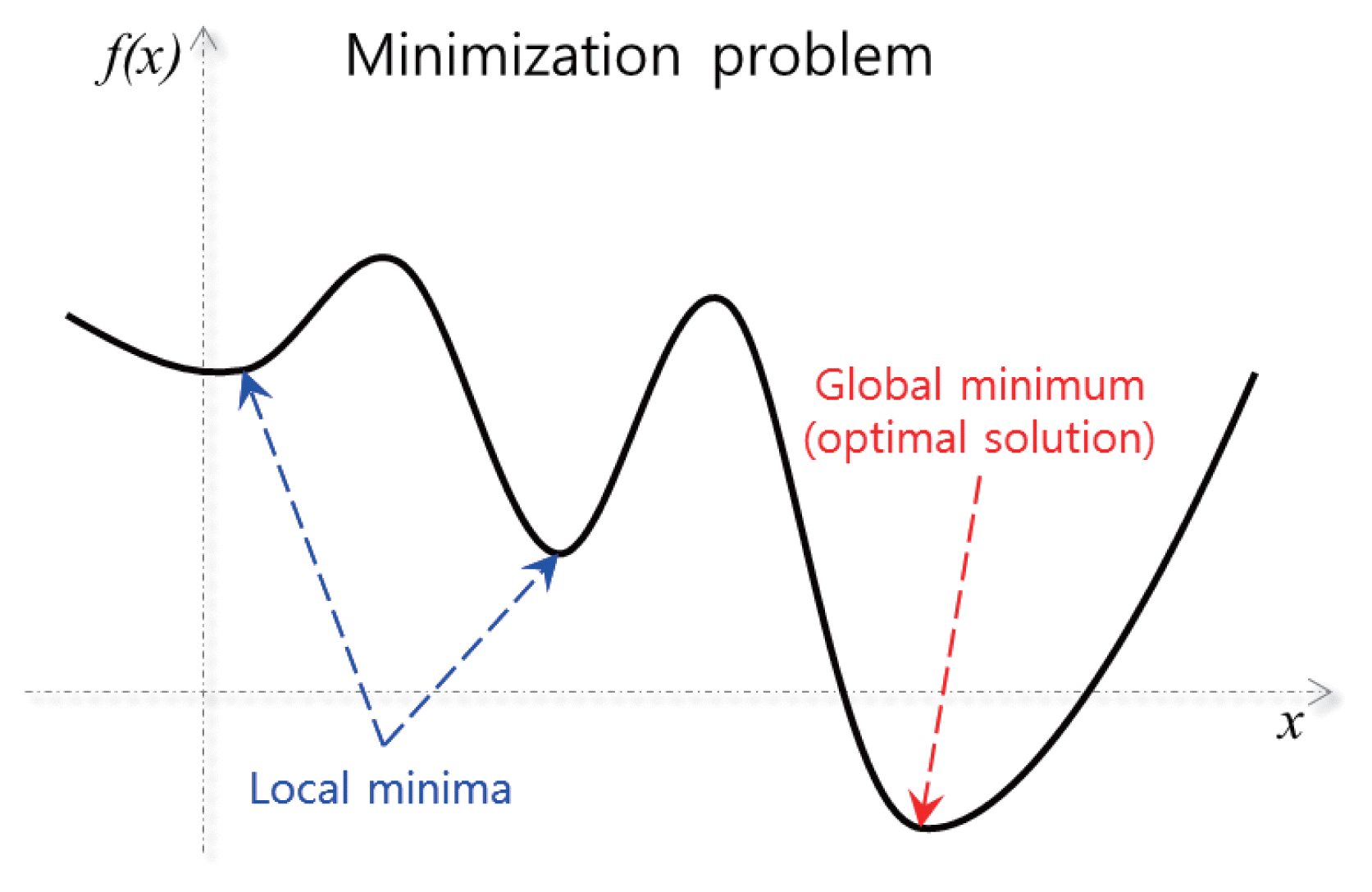
In a GA, solution candidates are treated as individuals, and these individuals form a population. Each individual has strings that correspond to the chromosomes in natural genetics. In the generation procedure, a new set of strings is generated by randomized selection, reproduction, crossover, or mutation from the past generation. Through a random procedure, the GA is not simple as general random search method. In the new generation procedures, the genotypes of genes are adapted to the environment to generate improved genes in the next generations using a fitness function. By iterating generations, individuals that have a mediocre fitness disappear, and those that have outstanding fitness are utilized in offspring production procedures. Consequently, only the individuals that have outstanding fitness will survive globally. This means that the result of a GA ultimately reaches the globally optimal solution with a high probability. Figure 1 shows the pseudocode of a generic GA, and Figure 2 shows an example illustrating the locally and globally optimal solutions. As shown in Figure 2, there are local minima and global minimum in an optimization problem. Only global minimum is the true optimal solution, and the others is not optimal solutions.
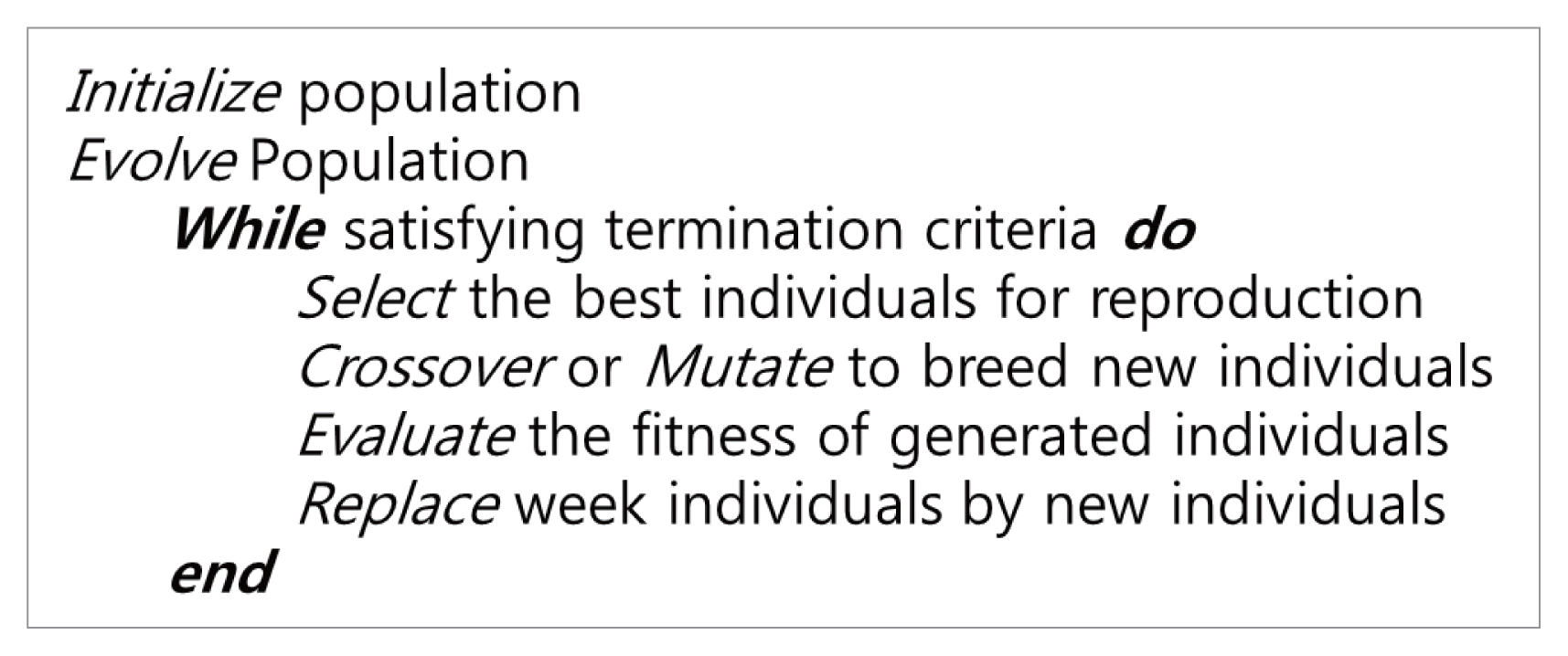
Pseudocode of a generic GA. In general, termination criteria can be the number of generations, individual tolerance and fitness tolerance.
2) Modified iterative genetic algorithm
Even though a GA is theoretically very good for searching for a globally optimal solution, it is not a perfect algorithm. Depending on the complexity of the problem, a GA also can find a local minimum as an optimal solution. Therefore, it is necessary to improve the GA to avoid local minima for several complicated problems.
There have been various studies of enhancements in GAs based on modifications of the original GA. Michalewicz et al. proposed a modified genetic algorithm (MGA) using specialized operators [16]. The operators are utilized in the mutation and crossover procedures to increase the convergence performance. However, MGA is developed based on systemic characteristics of control problems, it is difficult to be applied in general optimization problems. Several researchers have suggested iterative genetic algorithms (IGAs) to solve problems that have complicated variables associated with one another [17–19]. In these studies, GAs that optimize different values are arranged in cascaded stages, and a result from a node is utilized in next node as a constraint condition. IGAs are effective to optimize a system consisting of variables in complicated relationship, but the performance of optimization is not improved.
In this paper, a modified iterative genetic algorithm (MIGA), which has little in common with previous studies, will be presented. In the MIGA, several modifications have been applied to the IGA to modify the termination criteria to increase the probability to find globally optimal solution. In the GA, there are three termination criteria: the number of generations, individual tolerance, and fitness tolerance. However, the MIGA has four termination criteria. The number of generations and individual tolerance are akin to those of the GA. In contrast to other algorithms presented in previous studies, the MIGA utilizes a variable fitness tolerance and the number of iterations. For here, generation and iteration are intrinsic and systemic parameters of GA and MIGA. Individuals are corresponding to candidates of optimal detector positions, and fitness value means the value of optimization function described equation 4 that will be addressed in section 2.2.3.
To adjust the fitness tolerance, the end of GA procedure is supplemented with the competition procedure. In the competition procedure, the optimal result in a GA loop is selected and stored in a competition rank. By repeating each loop, the fitness of an individual ranked in first place among the competition results is fed back to the fitness tolerance. At the end of the MIGA, the one more GA loop is executed with the top-ranked individual as an initial condition to verify that the individual is the optimal solution. If the verification result is not optimal, the number of iterations is initialized, and entire MIGA is resumed with only the competition data. In short, the MIGA iterates GAs by the number of iterations to enhance the probability of reaching a globally optimal solution with adjustments of the fitness tolerance by competition and verifies the optimal solution at the end of the MIGA. The entire procedure is shown in Figure 3.
2. Calculation of detector positions for the system
1) Structural design
The structural design of an RPM for radioactive source localization is based on the external dimensions of container trailers. Standard ISO containers are 2.43 m wide and 2.59 m high and have two lengths, 6.06 and 12.2 m.1), In the case of trailers, the height of a flatbed trailer is commonly less than 1.40 m. Because vehicles move on the ground, the trailers frequently move from side to side but hardly up and down when they pass through an RPM. To consider these types of fluctuations, the spatial margins of the system are defined as follows; the height margin is 0.5 m, and the width margin is 0.65 m for each side. On the basis of this information, a basic structure of an RPM is designed. A conceptual design of the RPM is shown in Figure 4.

Conceptual design of an RPM for radioactive source localization. All detectors are NaI scintillator detectors that have a volume of 4×4×16 in3.
In this system, the number of detectors is equivalent to the number of input measurements. According to the number of detectors, the accuracy of source localization will be increased. However, it is not a sufficient solution to increase the number of detectors without other considerations because the relationship between the number of detectors and the localization accuracy is not simple. This relationship tends to be logarithmic rather than proportional. Because the number of detectors is highly associated with the performance of the system and budgetary constraints, the number of detectors must be determined on a case-by-case basis for each situation. However, the decision procedure will not be addressed because the details regarding this relationship are beyond the scope of this paper. In total, six detectors will be set on the RPM for our research.
NaI (TI) scintillator detectors with a volume of 4×4×16 in3 will be utilized for the RPM system. These detectors are also utilized in other RPM researches [5, 7]. If the active area is too small, the detection performance is poor, and if it is too large, it is difficult to specify the position of the detector. From this perspective, the NaI detector seems to be the appropriate choice and is the reason why it is widely utilized in RPM systems.
2) Inverse transport theory to define optimization problem
The measurements from detectors are utilized to localize a radioactive source. For a detector, a measured quantity of a source in a specific medium can be expressed as follows: [5, 11]
where
D = Measured quantity with a detector
A = the active area of a detector,
ɛip = the intrinsic parameter of a detector,
d = the distance between the source and the detector,
I0 = the intensity of the source,
μ = the absorption coefficient of the medium.
This equation is the simplest theoretical model. In this equation, uncertainties such as build-up effect, over estimation, measurement noise, and so on are ignored because mathematical modeling of them is too complicated. As presented above, a measurement is associated with the distance from a detector to a source. The distance is one-dimensional (1D) data, but the location is two-dimensional (2D) or three-dimensional (3D) data. Therefore, we have to acquire more measurements from other detectors to transform 1D data into 2D or 3D data. The relevant techniques have been commonly utilized in acoustic and sensor network studies [12–14]. The key aspects of these techniques is the solution of simultaneous nonlinear equations.
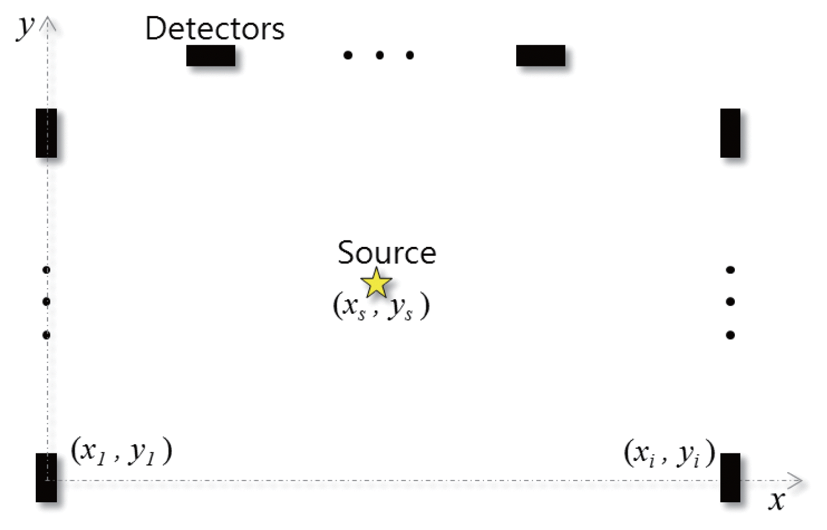
We define a radioactive source localization system as shown in Figure 5. The system consists of a structural frame, detectors, and their electronics. Each detector is fixed on a structure. Therefore, all detectors have their own fixed positions. In the case where a radioactive source is placed in the system, the number of measurements acquired may be equal to the number of detectors. Using the Pythagorean theorem, the distances between the sources and the detectors can be expressed mathematically. By substituting the equation for the distance into equation 1, a nonlinear equation concerning the position of a radiation source can be expressed as follows:
where
xs = the X coordinate of the position of the source,
ys = the Y coordinate of the position of the source,
xi = the X coordinate of the position of the ith detector,
yi = the Y coordinate of the position of the ith detector in the Cartesian coordinate system,
Di = measurement of the ith detector.
If all parameters concerning a detector and the radiation absorption are known, equation 2 can be expressed as nonlinear equations that have three identical unknown variables: xs, ys, and I0. This means that the position of the source can be calculated by solving a system of equations if the number of these equations is greater than three. It is possible to solve nonlinear equations even without the intensity of the source. The detector parameters can be confirmed by checking the specifications of the detector. In the case of the absorption coefficient, it varies with the medium that a radiation particle passes through. Because inhomogeneous media are quite complicated, only a homogeneous medium will be considered to simplify the problem in this research.
3) Problem definition
On the basis of the structural design of an RPM, the positions of each detector should be determined. The positions of the detectors should be considered according to the purpose of the system. In typical RPMs that are used to detect radioactive materials only, the positions of the detectors may not be very important because they are focused on the detection of radiation. However, the major purposes of these systems are the detection and localization of radioactive materials. From the perspective of localization, the contrasts among each measurement will affect the localization performance because the position of the source is calculated using the detector measurements. Therefore, the measurement contrasts should be maximized to increase the localization performance.
The other specifications of the structural design are already determined during the conceptual design, except for the positions of the detectors. These positions should be determined in the directions that maximize the contrasts of the measurements. Before defining an optimization problem, the source data should be established. In most cases in which an arbitrary radioactive source is contained in a container, the position of the source will be inside the container. Therefore, a region of interest (ROI) can be defined as an area that is identical to the external size of standard containers. Then, point sources that are regularly distributed within an ROI can be set as source data. In practice, cargo can’t be loaded to full container height because of limitation of the load weigh. However, just for simplification, the distribution of source points was assumed to be uniform. In this paper, an array of 11×11 point sources is utilized as the data. All sources are monoenergetic, and the intensity of a source is 1×10⁶ gamma rays·s−1.
As mentioned in section 2.2.2, the position of the source can be calculated if all other parameters are known values. To define the problem, all parameters are defined as follows. The inner space of the RPM is assumed to be a homogeneous medium. The absorption coefficient of the medium is chosen to be 10−4 cm−1, equivalent to the microscopic cross section of air. Each detector is assumed to have an active area of ~412.9 cm2 and an intrinsic efficiency of 10% for simplification. These values are reasonable for NaI scintillator detectors [5].
With the defined source data and parameters, equation 1 can be expressed as a function of the unknown detector positions as equation 3. In this equation, the unknowns are marked by star symbols.
The simultaneous calculations of the differences for 121 sources is equivalent to the case in which the measurement differences of each detector for a strong source located at the center of the ROI are calculated. Therefore, the differences should be calculated on case-by-case basis for each source. To maximize the contrast of the measurements regardless of the location of a source, the following objective function is defined:
where
where
m = the number of sources,
n = the number of detectors,
Di = measurement of the ith detector according to equation 1,
(Dij)k = total difference in the measurements between the ith and jth detectors for the kth source.
In optimization problems, maximization can also be represented as minimization by attaching a negative sign to the objective function. The reason why Dij is divided by 2 is to countervail the overlap between two identical differences such as D12 and D21. By substituting the Di and Dj terms in equation 4 with equation 3, the objective function can be represented with the unknown detector positions.
The equality and inequality constraints of this problem are related to the structural frame of the RPM. Six detectors will be installed in this system, as mentioned above. The frame consists of three beams on the left, right, and top sides. On each side of the frame, two detectors can be assigned: detectors 1 and 2 to the left, detectors 3 and 4 to the top, and detectors 5 and 6 to the right sequentially. For the left- and right-side detectors, the x positions are fixed on the frame. The y positions are adjustable but limited to the height of the frame. For top-side detectors, the x positions are adjustable but limited to the width of the frame. The y positions are fixed on the frame. When each position of the detectors is represented by two vectors X and Y, these equality and inequality constraints can be written with vectors and matrices as follows.
1) Equality constraints
2) Inequality constraints
In equations 5 and 6,
where
A = the matrix for selecting the left- and right-side detectors,
B = the matrix for selecting the top-side detectors,
W = the width of the RPM frame,
H = the height of the RPM frame,
xi = the X coordinate of the position of the ith detector,
yi = the Y coordinate of the position of the ith detector in the Cartesian coordinate system.
Results and Discussion
1. Performance evaluation of the MIGA
The optimization problem defined in section 2.3.2 was solved by two algorithms—the GA and MIGA. These algorithms were implemented in a MATLAB environment to compare their performance. In this section, the optimization results and analyses will be presented sequentially.
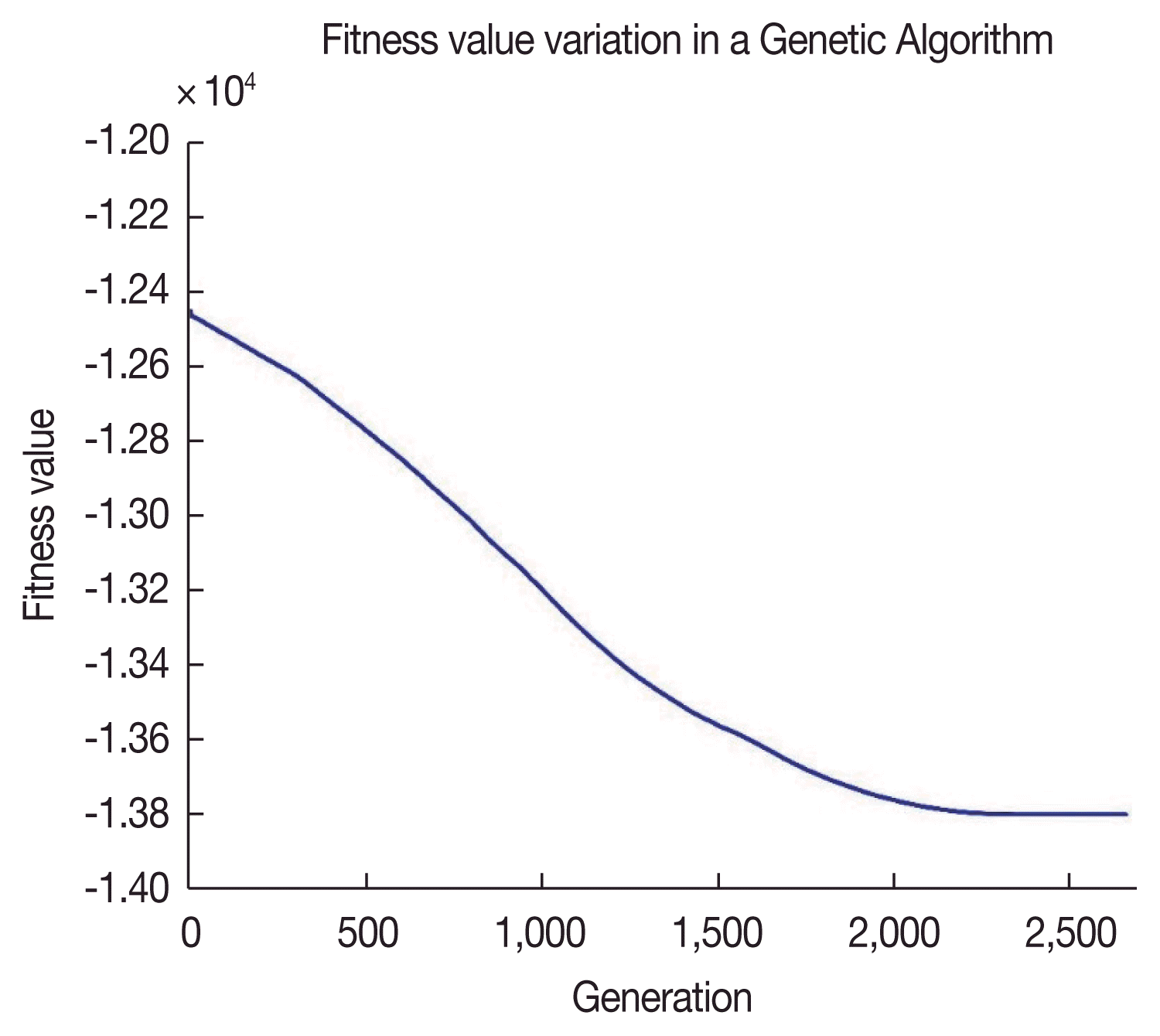
A GA is an effective algorithm for finding a globally optimal solution, but the result might be a locally optimal solution depending on the complexity of the problem. Figure 6 shows the variation in the fitness value for each generation. For simulation, the number of generation is set to 2,000, and individual tolerance and fitness tolerance are equally set to 1×10⁻²⁰. At the beginning of the GA, the fitness value decreases rapidly. This means that the GA searches the optimal solution effectively. Then, the fitness value converges. This shows how the GA finds the optimal solution.
In the MIGA, the competition, iteration, and verification procedures are added to increase the optimization performance. Figure 7 shows the fitness value versus the number of iterations for the MIGA. To solve the defined problem using the MIGA, the number of iterations is set to 1,000. As shown in this figure, calculation results for each iteration are not constant. This shows one of the weaknesses of the GA; all of the points in Figure 7 represent the optimization results from each GA loop. However, only the points on the red dashed line that represent the minimum fitness values are real optimal solutions, and the others are local minima. This means that we cannot know whether the solution is a globally optimal solution when using the GA only. Therefore, it is necessary to utilize the iteration and competition procedures to increase the probability of finding globally optimal solutions.
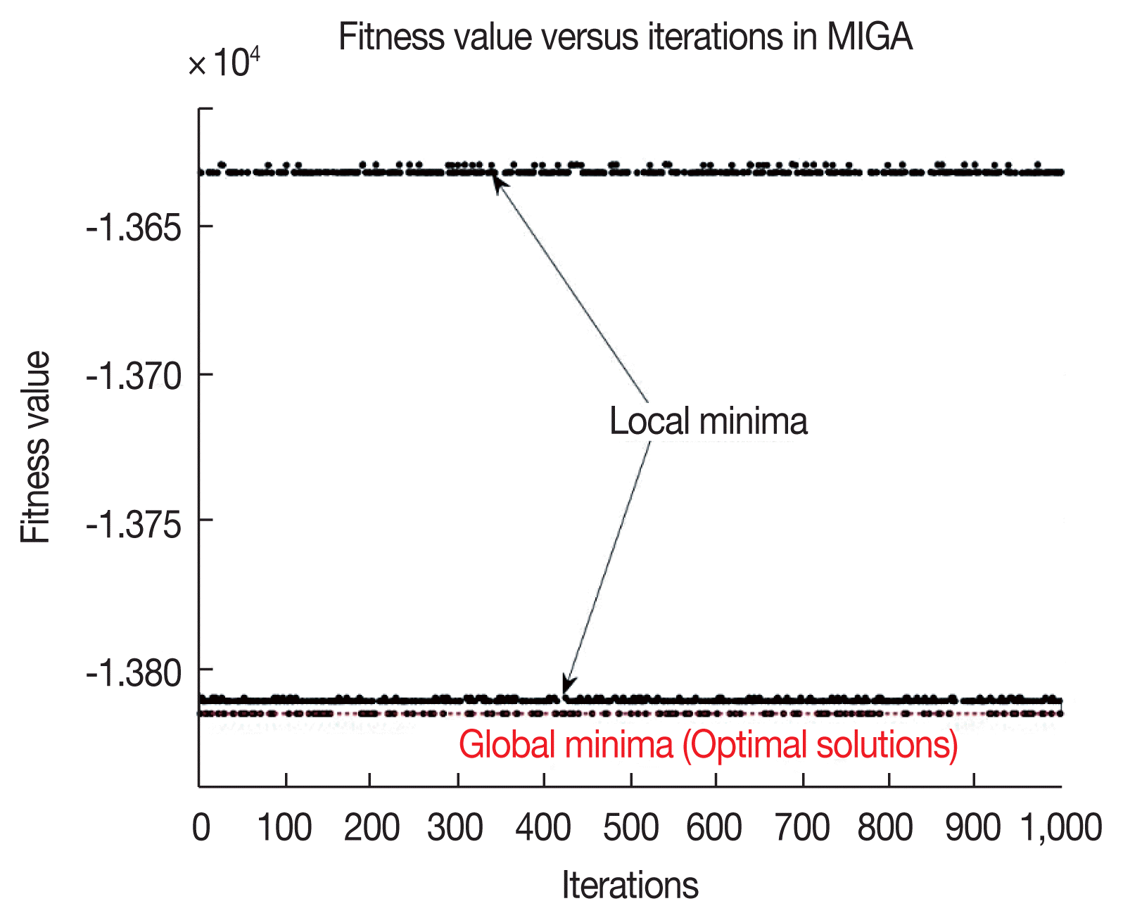
Fitness value versus the number of iterations for the MIGA. Each point represents the optimization result from the GA, but only the points on the red dashed line are optimal solutions.
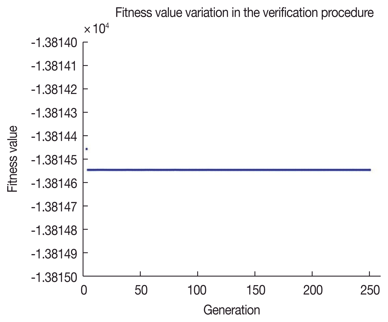
At the end of the MIGA, the verification procedure is added to confirm whether the final result is globally optimal. In the verification procedure, the GA is executed once again with the final result as an initial condition. If the result is a globally optimal solution, the verification result will be identical to the initial values themselves. Figure 8 shows the variation in the fitness value during the process of verification. Although the variations in the fitness values are almost zero, the GA repeats the generation process 263 times. This shows that the GA attempts to find another globally optimal solution.
Figure 9 shows a schematic of optimization using the MIGA. The basic frame of the RPM is described by the black bold line. A container (ROI) and flatbed trailer are described by red and green dashed lines, respectively. The cyan, red, and blue stars represent the source information, the optimal positions of the detectors calculated by the MIGA, and the trisection points of the ROI, respectively. Because the fact that the point sources are uniformly distributed inside of ROI is utilized as source information, we expect the result to be related with the area of the ROI. Therefore, the trisection points were considered as estimated optimal positions. However, an optimal solution is found, which has lower fitness value than the estimated solution by 175.5565. An RPM system has been designed using this optimization result. We also tried to solve this problem using GA, but we cannot find globally optimal solution that is found by MIGA. Table 1 summarizes the estimated solution, local solution using GA, optimal solution using MIGA, and their fitness values. In Table 1, each solution is represented by the position (X, Y), and all values are presented in units of millimeters (mm).
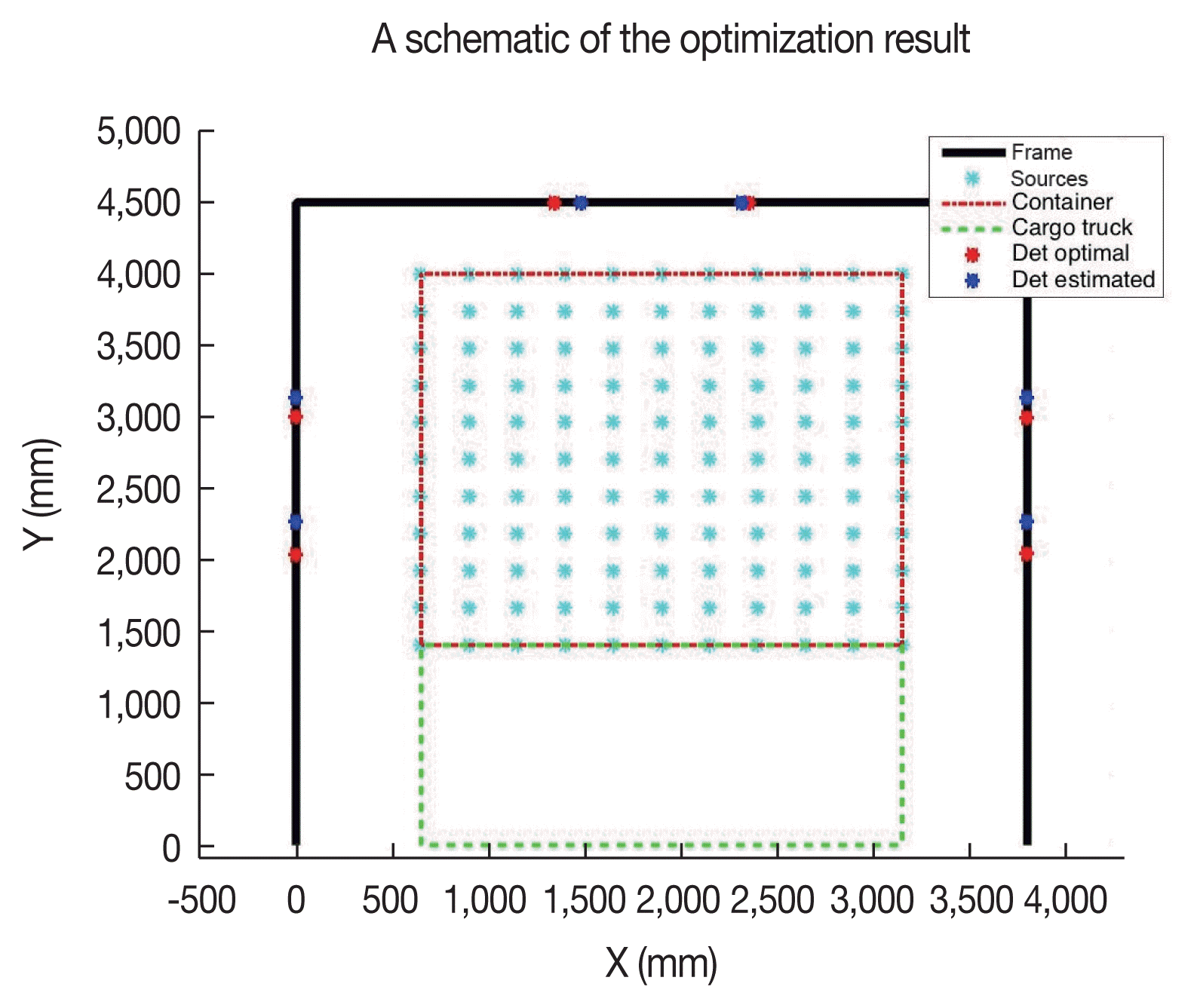
Schematic of the final optimization result using the MIGA with 100% loading rate source data. The fitness value of the optimal solution is lower than that of the estimated position by 175.5565.
In common sense, detectors should be located in symmetry. However, the case that the positions of detectors are located in asymmetry has higher fitness value than symmetric case as shown in Figure 9 and Table 1. We thought that this result may cause owing to the definition the objective function. We defined the objective that maximize the contrast of detector measurements. In perspective of maximizing the contrast, the contrast is getting larger in unbalanced condition than balanced condition.
Conclusion
In this paper, a machine learning algorithm was utilized to calculate positions of detectors for radioactive source localizing RPM system. To calculate detector positions, an optimization problem was defined. To achieve a reliable solution, the MIGA was suggested by modifying a GA with supplemental iteration, competition, and verification procedures. The GA and MIGA were implemented using MATLAB, and their performance was analyzed. In the case of the MIGA, the result was analyzed systematically. According to resulting optimization analyses, all supplemented procedures help to find a globally optimal solution.
This paper is a preliminary step for the development of an intelligent RPM system that can detect the position of a radioactive source using machine learning algorithms. To apply machine learning to RPM systems for source localization, it should be designed to maximize the performance of the system in accordance with the characteristics of the algorithms.
In typical pattern recognition problems, one of the most essential research fields in machine learning algorithms, all input data are transformed into features that represent the characteristics of all patterns, and machines are trained by features to recognize an object. To increase the performance of a machine for pattern recognition, many samples that consist of clearly distinguishable features should be supplied.
To implement a high-performance intelligent localization system, the information produced by the system should be distinguishable because features are generated by the information. In the case of an intelligent RPM, measurements from the detectors will be utilized as the information. Therefore, it is important to design a system so that it can generate distinguishable detector measurements. In short, the contrasts of the detector measurements should be clear. For this reason, an optimization problem was set up to maximize measurement differences in each detector.
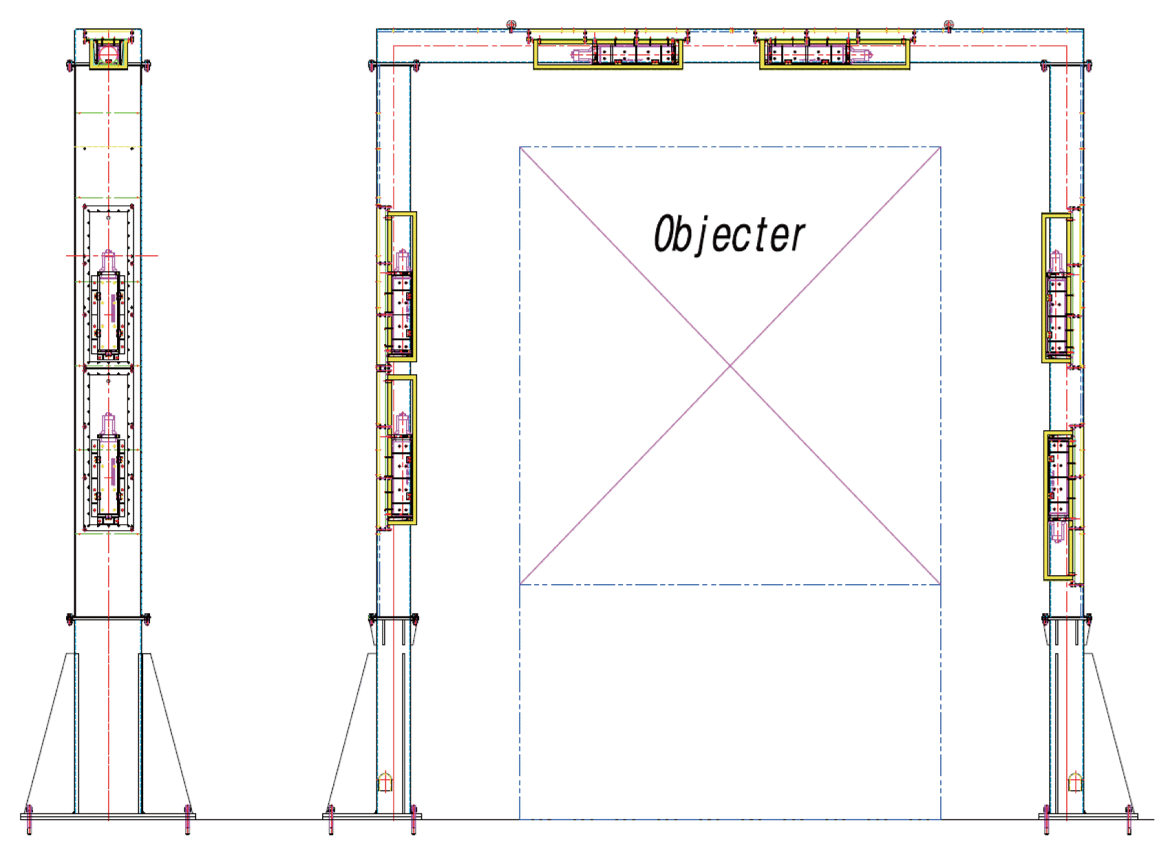
On the basis of this study, an RPM has been designed and will be fabricated. Figure 10 shows a mechanical drawing of the designed RPM. However, an evaluation of the localization performance with this optimization result cannot be conducted immediately because another machine learning algorithm for localization should be implemented. As the next step of this work, an intelligent RPM system for radioactive source localization using a machine learning algorithm will be researched by utilizing this designed RPM system. Then, the localization performance of this system will be evaluated.
Acknowledgements
This research was a part of the project titled “Research on fundamental core technology for ubiquitous shipping and logistics” funded by the Ministry of Oceans and Fisheries, Korea, contract No. D10802514H380000110. The authors sincerely appreciate for the support.
Notes
ISO 6346 Freight Containers-Coding, Identification and Marking.
